Revenue, GMV, ARPU, order value — money metrics almost never look like a neat bell curve. A handful of whales sit far to the right; most users spend little or nothing. If you feed that raw distribution into a standard mean comparison, you pay for it: noisy estimates, fragile p-values, and “wins” that disappear when one big spender lands in the wrong bucket.
Log-transforming the metric is the classic fix. This guide explains why it works, what the formulas mean, how the distribution changes, and how to read the result as a percent lift your product team can actually use.
Why money metrics are right-skewed
Spending is multiplicative, not additive. Someone who “buys a bit more” often buys proportionally more — and a small share of users accounts for a large share of revenue. That process naturally produces a long right tail. In practice, revenue-per-user often looks approximately log-normal: the log of the metric is roughly normal, while the raw metric is not.
A typical raw histogram looks like this — mass near zero / low spend, then a thin tail of high spenders:
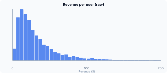
Under that shape, the arithmetic mean is pulled by outliers. Sample means jump around from experiment to experiment. Variance estimates blow up. Classical t-tests still “work” asymptotically by the CLT, but in finite samples — especially with heavy tails — they lose power and become sensitive to a few extreme observations.
What the log transform does
Take the natural logarithm of each observation (any base works; natural log is the usual choice in stats software):
where \( x_i > 0 \) is revenue (or GMV, order value, …) for user \( i \)
Multiplicative gaps on the original scale become additive gaps on the log scale. Doubling spend is a fixed shift of \( \log 2 \), whether you went from $10 → $20 or $1,000 → $2,000. That compresses whales, stretches the dense low-spend region, and — when the data are roughly log-normal — produces an approximately symmetric, near-Gaussian distribution:
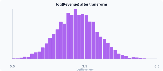
Rule of thumb: if a few users can swing the mean by tens of percent, you almost certainly want a transform (or a robust / CUPED / winsorized approach) before trusting a raw-mean A/B test.
Zeros and log(x + c)
log(0) is undefined. If your metric includes non-paying users (revenue = 0), common options are:
- log1p: \( y = \log(1 + x) \) — defined at zero, almost \( \log x \) for large \( x \).
- Two-part analysis: test conversion (paid vs not) separately from spend among payers (then log the positive amounts).
- Filter to the relevant population: e.g. log(order value) only among purchasers, if that matches the decision.
log1p — safe when \( x_i \ge 0 \)
Pick the zero-handling strategy before the experiment and stick to it. Switching after peeking at results is a classic way to inflate false positives.
Why this is statistically the right move
You’re not “faking” the data. You’re matching the analysis to the generative structure of the metric.
1. Log-normal model
If \( X \) is log-normal with parameters \( \mu \) and \( \sigma^2 \):
Then comparing means of \( \log(X) \) is comparing the natural parameters of the distribution. The mean of \( \log(X) \) is also the log of the geometric mean of \( X \) — a more stable summary of multiplicative data than the arithmetic mean.
2. Effects you care about are relative
Product changes usually move revenue by a percent, not a fixed dollar amount for every user. On the log scale, a constant additive shift \( \delta \) means a multiplicative change of \( e^{\delta} \) on the original scale:
Example: \( \delta = 0.05 \) → \( e^{0.05} - 1 \approx +5.1\% \)
That maps cleanly to how stakeholders talk (“+5% revenue”) and to how most uplift models are specified.
3. Better-behaved variance → better power
After the transform, sample variance is less hostage to a few outliers. Confidence intervals shrink for the same n. You detect real relative lifts with fewer users — or with the same users, more reliably. That is the practical payoff, not a mathematical curiosity.
How to run the A/B test on logs
- 1. Define the unit and metric — usually per user, e.g. revenue in the experiment window.
- 2. Handle zeros up front — choose log(x), log(1+x), or a two-part design; pre-register it.
- 3. Transform — compute y = log(…) per unit in control and variant.
- 4. Test on y — t-test, regression with CUPED, or your usual stack on the transformed metric.
- 5. Convert the effect — \( \hat\delta = \bar y_B - \bar y_A \), percent lift \( = e^{\hat\delta} - 1 \).
- 6. Convert the CI the same way — \( [e^{L} - 1,\; e^{U} - 1] \).
Do not exponentiate the p-value or treat exp(mean of logs) as if it were the arithmetic mean of revenue. The geometric mean and the arithmetic mean answer different questions. For decision-making on multiplicative lifts, the log-scale comparison is usually the one you want; if finance needs expected dollars per user, report that separately (or use a model that targets E[X] directly).
Common mistakes
- Logging after aggregation. log(sum of revenue) ≠ analyzing per-user logs. Transform at the analysis unit, then average.
- Mixing scales in one sentence. “Mean log-revenue up 0.04” is not “+$0.04.” Convert to percent when you communicate.
- Ignoring zeros. Silently dropping zeros or using log(x) on a metric that includes them will crash or bias the analysis.
- Winsorizing instead of thinking. Caps can help, but they answer a different estimand. Log + relative lift is often cleaner for money.
- Forcing log on already-symmetric metrics. Conversion rates and many count metrics don’t need this; use the right family (binomial, Poisson, etc.).
When not to log-transform
Skip or rethink the log when:
- The metric is already close to symmetric and light-tailed.
- You specifically need the arithmetic mean in dollars (e.g. accounting total), and you’re prepared for heavier tails — then use methods aimed at E[X] (e.g. gamma GLM, robust SEs, bootstrap), not a silent log.
- Effects are thought to be additive in dollars for every user (rare for spend, more common for some fee or credit mechanics).
Summary
Money metrics are right-skewed because spending is multiplicative. Logging pulls the distribution toward normality, stabilizes variance, and makes treatment effects interpretable as percent lifts via \( e^{\delta} - 1 \). Handle zeros explicitly with log1p or a two-part design. Report results on the percent scale, keep the analysis plan fixed before launch — and your revenue experiments will stop being dominated by whoever the whales were that week.
Analyze skewed metrics the right way
AB-Labz picks suitable methods for your metric type — including transforms and clear effect-size reporting — so revenue tests don’t get hijacked by outliers.